Two new PyPI packages

Long time without posting… Let’s try to get back on track!

I have created two simple packages implementing useful probability distributions.

The LogUniform package provides the log-uniform and the modified log-uniform distributions, while the kumaraswamy package provides an implementation of the Kumaraswamy distribution.

Both packages implement similar APIs to the scipy.stats package.

LogUniform

The log-uniform distribution, often called the reciprocal distribution (Wikipedia) or, in some contexts, the Jeffreys prior, is commonly used as a prior for parameters which vary over several orders of magnitude.

Its probability density function (pdf) is given by

The two parameters \(a\) and \(b\) correspond to the lower and upper bounds of the support.

Here is what it looks like, for \(a=1\), \(b=100\)

The modified log-uniform distribution is a modified version of the log-uniform distribution (!), which extends its support to include \(x=0\). The pdf is

with \(x_0\) (sometimes called the knee of the distribution) and \(b\) as parameters. The support of this modified distribution goes from \(0\) to \(b\).
It looks like this, for \(x_0=1\) and \(b=100\)

Ok, now some code. To use the LogUniform implementation¹, we would first install the package

$ pip install LogUniform

and then use it from Python as

import loguniform
dist = loguniform.LogUniform(a=1, b=100)

The dist object has methods much like those of a scipy.stats distribution:

dist.pdf(x)  # Probability density function evaluated at x
dist.cdf(x)  # Cumulative distribution function (cdf) evaluated at x
dist.sf(x)   # Survival function (1 - `cdf`) evaluated at x
dist.ppf(p)  # Percent point function (inverse of `cdf`) evaluated at p

and a few extra properties:

>>> dist.mean
21.497576854210962
>>> dist.mode
1
>>> dist.std, dist.var
(24.96961794931886, 623.4818205349466)
>>> dist.skewness, dist.kurtosis
(1.4283873461330863, 1.0492789588735452)

The same thing for the modified log-uniform:

dist = loguniform.ModifiedLogUniform(knee=1, b=100)

>>> dist.pdf(0)
array(0.21667907)
>>> dist.cdf(dist.b)
1.0

>>> dist.mean
20.667906533553168
>>> dist.mode
0
>>> dist.std, dist.var
(25.210415697969275, 635.5650596644156)
>>> dist.skewness, dist.kurtosis
(1.430935496096598, 1.0573553176553114)

kumaraswamy

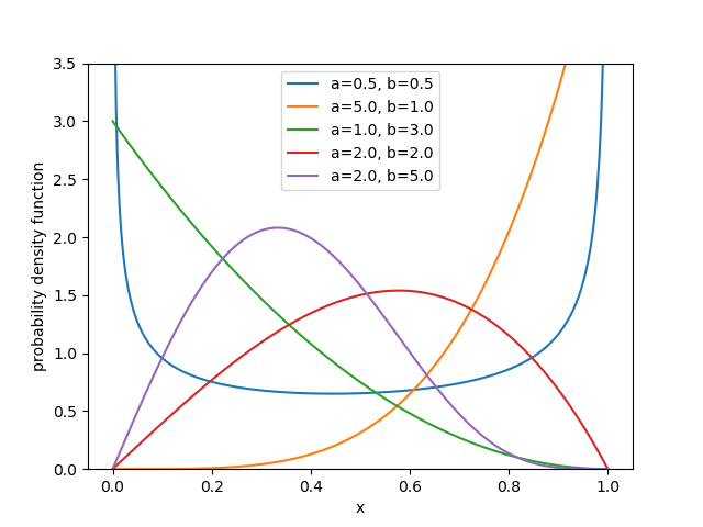
The Kumaraswamy distribution (see Wikipedia) is a little known family of continuous probability distributions defined on the interval [0,1]. It’s particular because of the similarities to the Beta distribution, and because (unlike the Beta) its pdf and cdf are easily evaluated.

The pdf is given by

with \(a\) and \(b\) the two shape parameters. Depending on the values of these parameters, the distribution can have a range of different shapes:

In order to use the kumaraswamy package, we first install it

$ pip install kumaraswamy

and then use it from Python, much like before

import kumaraswamy
dist = kumaraswamy.kumaraswamy(a=.5, b=.5)

with the same methods and properties now available in dist.

To finish, one extra method shared by the three distributions provides random samples:

>>> dist = loguniform.LogUniform(a=1, b=100)
>>> dist.rvs(3)
array([99.88014766, 28.10705983, 34.18542689])

>>> dist = loguniform.ModifiedLogUniform(knee=1, b=100)
>>> dist.rvs(100)
array([1.30284699e+01, 3.26860325e+01, 1.10717848e+00, 8.66021941e+01,
       3.66928668e+01, 6.40408882e+00, 1.50455730e+01, 3.90749222e+01,
...

>>> dist = kumaraswamy.kumaraswamy(a=.5, b=.5)
>>> dist.rvs()
0.4416781513613892

wrap up

That’s it, two simple packages implementing three probability distributions for some of your statistical needs.

Let me know in the comments if this is helpful, wrong or super-duper cool.